I tried to optimize a tour of the most beautiful villages in France (traveling salesman problem) like a quantum computer, but it didn’t work in the end. But I learned a lot.
Quantum computers already exist.
Quantum computers are becoming so commonplace that they’ve recently been featured in the general news. The MIT Technology Review has listed it as one of the technologies to watch in 2017.
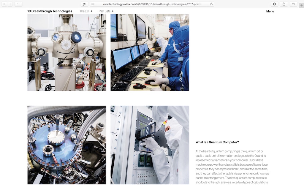
出所:10 Breakthrough Technologies 2017: Practical Quantum Computers – MIT Technology Review
In my day and age, I thought that quantum computers would never come to fruition. However, the announcement of the research by Google and NASA on December 8, 2015 was probably the biggest shock in recent years. I remember hearing this news and being amazed that quantum computers had actually been developed to this extent.
【主なメディアでの関連ニュース(英語メディアのみ)】
もちろん量子コンピューターが実在している自体も驚きでしたが、それだけでなく、ごく限られた条件とは言え、現時点でも従来型のコンピューターよりも1億倍も速いということにも驚きました。ただ正直な処、1億倍といってもピンとこないですよね。ざっくりしたたとえですが、[highlight]「これまで1億秒=3年2ヶ月くらいかかっていた計算をたったの1秒でできてしまう」[/highlight]ということです。こう考えると確かにものすごいことです!もっともそんな3年もかかる計算って一体何?とは思いますけどね笑。
What is the annealing that led to the realization of quantum competitor?
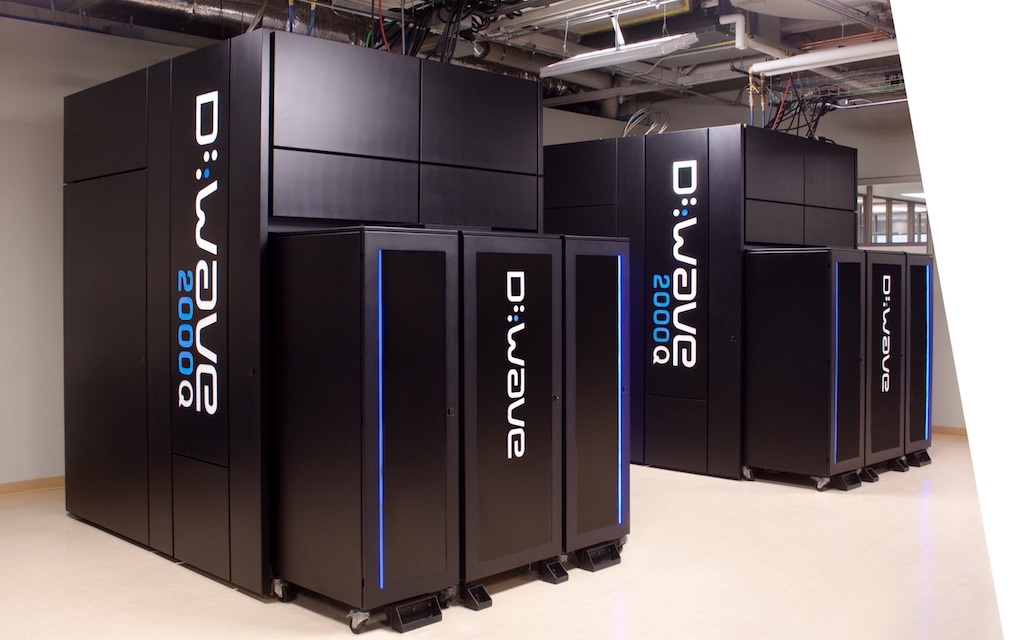
さて、このときにGoogleとNASAが使っていたのが、D-Waveシステムと呼ばれる量子コンピュータです。この量子コンピュータは、これまで長年研究されてきた「量子ゲート方式」ではなく、「量子アニーリング方式」というもので構築されているのが最大の特徴です。
Quantum annealing is the use of quantum statistical mechanics to solve combinatorial optimization problems and to perform sampling. You should be able to understand the basic mechanism if you have knowledge of physics at undergraduate level, especially statistical mechanics and quantum mechanics.
If you want to know more about it, the page of Mr. Nishimori, professor of Tokyo Institute of Technology, who is the leading researcher of this quantum annealing research, is the most helpful. I think his site is a must for you to know this world.
参考サイト:量子アニーリング(西森秀稔)
For a more general review, the following book, also written by Nishimori, is also very helpful.

Amazon.co.,jpへのリンク: 量子コンピュータが人工知能を加速する
It was very helpful for me to know the trend especially in recent years.
The company that created the quantum computer
そして、量子アニーリングのロジックを実現するコンピュータを実際に作ってしまったが、こちらのカナダのとあるベンチャー企業[highlight]「D-Wave Systems Inc.」[/highlight]。やはりというか物理学者が起業したとのことです。
In the example paper by Google and NASA, they refer to the computation using this computer as “Physical Quantum Anealing”. The reason why it is called “physical” can be better understood by comparing it with the quantum Monte Carlo method, which I will explain later.
So far, it seems that quantum annealing can handle and calculate only a few algorithms such as combinatorial optimization and cluster decomposition. In the future, it is expected to have the potential to show its power in artificial intelligence and machine learning, especially in deep learning. After all, it is 100 million times faster. I would like to expect that various applications will be created by analogy with existing physical theories.
Applied technology and software for quantum computers are also being developed.
量子コンピュータD-Waveの登場により、その活用方法について考え始めた会社もすでに存在、[highlight]「1QBit」[/highlight]という会社です。こちらもカナダの会社だとか。
写真の出所および詳細はこちら:Home – 1QBit
この会社のウェブサイトでは、すでにいくつかホワイトペーパーを後悔しています。直近のリリースではファイナンス関係が続いていることは注目です。例えば「Quantum-Inspired Hierarchical Risk Parity」ではアセットアロケーションの話題を、そして「Finding Optimal Arbitrage Opportunities Using a Quantum Annealer」では為替の裁定取引の話題を取り上げています。ファイナンスは、量子コンピューターの応用分野の有力候補のひとつのようですね。ビジネスにもつながりやすいですからね。
In fact, the example paper from Google and NASA also claims to have measured speed differences between computers and calculation methods based on portfolio optimization problems.
(ちなみにこの論文をくまなく読んでいくとこの論文では用いなかったが、彼らはこのポートフォリオ最適化問題をもっと高速に解けるアルゴリズムを発見したらしいです。「 量子コンピュータが人工知能を加速する」より)。
If it’s finance, I’d like to dig a little deeper because I’m very interested in it because I work in that industry, but I don’t want to write about things that are too close to my work these days because it can be troublesome.
You can do quantum computer-like things at home
そんなワクワクなD-Waveシステム、さすがに現時点では個人でこれを使うことはできませんが、一方で量子アニーリングの概念は、何もこのコンピュータでなくても、従来型コンピュータ、つまりいま手元にあるPCでも実現することはできます。それは、[highlight]量子モンテカルロ法(経路積分量子モンテカルロ法, Quantum Monte Carlo Simulation)を利用する方法[/highlight]です。
In addition, as a method for solving combinatorial optimization problems, a rather classical method called simulated annealing, which is based on an analogy with physical theory, has been known.
例の前述のGoogle&NASA論文によれば、ビット数があまり大きくなければ、古典的なアニーリング、すなわちシミュレーティッドアニーリング(SA)の方が、量子モンテカルロ法(QMC)による量子アニーリングよりも早く計算できゆようですが、ビットサイズが1,000近くになると量子モンテカルロ法の方が速くなるようです。
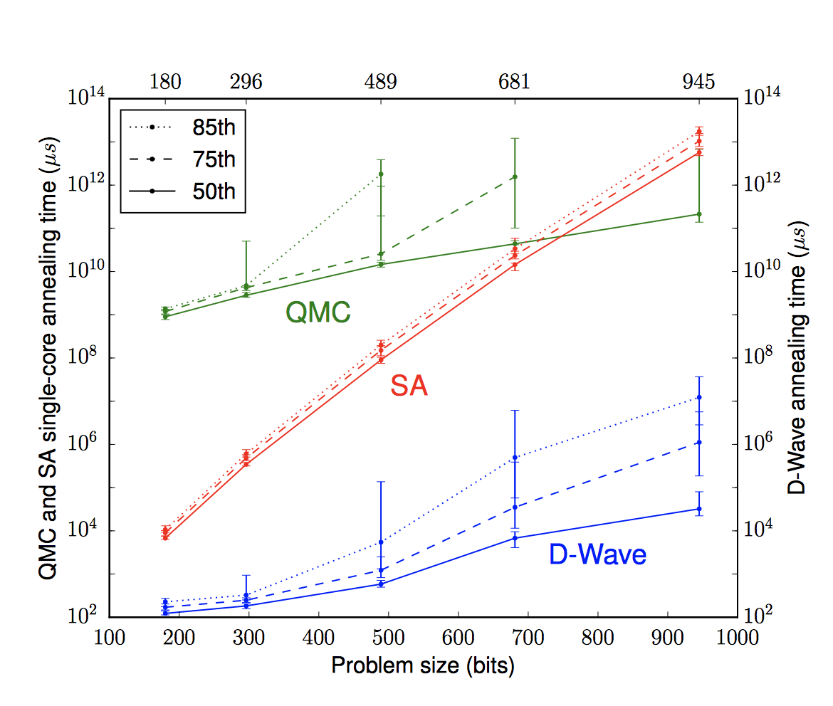
出所:What is the Computational Value of Finite Range Tunneling?より
In other words, using the quantum Monte Carlo method, even a conventional computer can take advantage of its speed as the number of bits increases. This is similar to hadoop, which is not so good for small data, but powerful for big data.
Incidentally, I think the 100 million times faster figure in the example comes from a comparison between simulated annealing and physical quantum annealing with D-Waves. It’s also interesting to note that the difference in the speed of the quantum Monte Carlo and D-Waves results as you increase the number of bits is not very dependent on the number of bits, as opposed to the rapid increase in computation time for simulated annealing.
Of course, it’s better to use D-wave, but even if you can’t use D-wave, it’s possible to study quantum annealing. At the very least, it’s a great way to explore the possibility of generalization beyond combinatorial optimization and cluster analysis. It’s easy for anyone to do.
Trying to optimize travel plans at home, quantum computer style
In order to deepen my understanding of quantum annealing, I decided to play with the quantum Monte Carlo method. As a concrete material, I chose the problem of making an optimal route for a tour of the most beautiful villages in Italy, which I have visited before.
The sample I calculated before was “Tour of Italy’s Most Beautiful Villages, Southern Italy & Sicily”.
For this test, we decided to run the quantum Monte Carlo program not on the most beautiful villages in Italy, but on the most beautiful villages in mainland France, which is the main focus of this site. We will then compare the results with those of our previous program to see how accurate the Monte Carlo method is and how long it takes to solve.
The calculations can be done in Python
This quantum Monte Carlo method using a conventional computer can be easily implemented in programs such as R or Python. I found some concrete Python code here. There is also a brief explanation of quantum annealing, which is a good refresher for those who don’t have prior knowledge.
参考にしたサイト:量子アニーリングで組合せ最適化
Basically, we’ll use the code as written here, but I personally didn’t like the word cost in some parts of the code, and the correspondence between the distribution function (in the logic explanation) and the function in python was not clear at first glance. Then, I rewrote the cost part of the code to match the shoulder of the exp of the distribution function (the content enclosed by -β) as follows
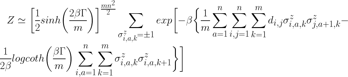
In short, since the effective energy when quantum effects are taken into account can be expressed as
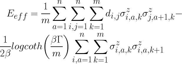
I just made sure this was reflected in the code for clarity. What we are trying to calculate is the same.
Use location information acquired with Google direction API
As before, we used Google Map API to create distance and travel time matrices for the distance and travel time between villages. It is possible to use the API to get the data each time, but as I recall, using the API too much in a short period of time might cause an error, so I decided to run the API only for the necessary amount in advance and create the distance and travel time matrix between each village first.
In reality, I think it’s better to optimize the travel time than the travel distance, so I’ll find the solution that minimizes the travel time. This can also be obtained from the API, because the travel time of Google Map is really accurate.
The json file containing the distance between two points, travel time, travel route, and other information acquired in advance this time has 158 targets (Charles de Gaulle Airport in Paris was added as the starting point), so the number of location information json files that must be acquired is 158 x 157 / 2 = 12,403.
However, Google Maps Direction API is free up to 2,500 requests per day, and if you use more than 2,500 requests, it costs $0.5 per 1,000 requests. It costs about 500 yen, but it’s a hobby.
In addition, this time, instead of simply displaying a straight line between cities as before, I also reflected the actual travel route on Google Maps. In other words, the line connecting each village within the optimal route is decoded from the json routes.legs.steps[i].polyline.points value obtained from the Google Maps Direction API, and then the Google Maps javascript API I tried to run the polyline option.
詳しい使い方はhttps://developers.google.com/maps/等を参照にしてみてください。
Googleのサイト:Interactive Polyline Encoder Utility
In addition, there are many other information on the web. You can google “Google Maps API encode data decode”. By the way, I used the following site as a reference.
参考にさせていただいたサイト:Google Static Maps APIの使い方まとめ!画像地図を作ろう!
So, first of all, here is the result of the optimized route calculated by the previous program.
最適化ルート従来版:フランスの美しい村巡り 最適ルート2017年
The total travel time is 614,345 seconds = 7 days, 2 hours, 39 minutes and 5 seconds.
However, in this program, the start point is not the goal point. It looks like I need to improve the code to make it work, but I gave up this time because it seems to take a little time with my code writing ability.
Quantum Monte Carlo results took too long to compute
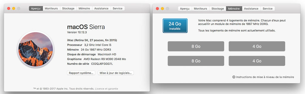
Well, I wanted to tell you the result, but it took too much time and I almost gave up the calculation in the middle, but I managed to get it. While it took only a few seconds by conventional programming, it took 10 or 20 hours by imposing various parameter conditions on the calculation by quantum Monte Carlo. The PC I used for the calculation is iMac 27inch, and the specs are as follows.
If it takes this much time, it is not comparable to the method (*probably simulated annealing) that I used before for the Italian village optimization. It is not useful at all at this level. I can also say that the python library I used 3 years ago for my tour of beautiful Italian villages is too amazing.
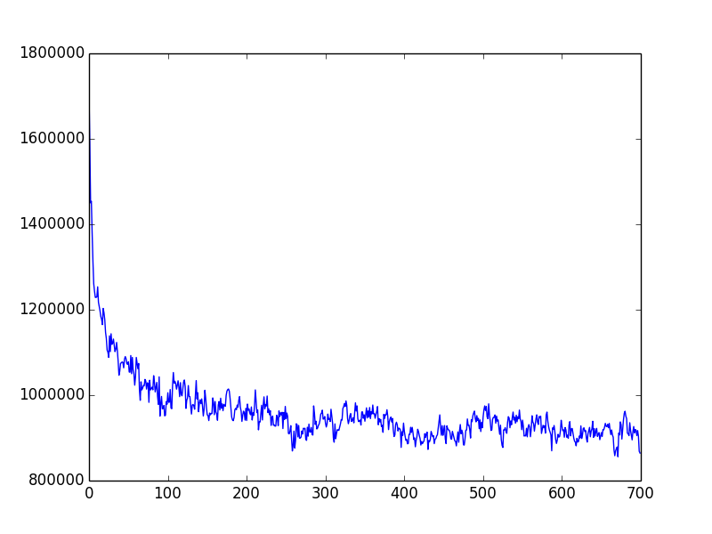
Anyway, no matter how many times I change the parameters, the time it takes to go around all the villages never goes below 850,000 to 900,000 seconds. It falls steadily down to about 100,000 seconds, which means that the travel time becomes smaller, but from there on, no matter how many times I run Monte Carlo, I can’t move forward. The previous one was 610,000 seconds, so the length of the process is about 1.5 times longer. It’s not good at all.
By the way, the following graph is the result of my quantum Monte Carlo calculation. The horizontal axis is the number of times the magnetic field is adiabatically set to zero (the number of annealing iterations?). and the vertical axis is the total travel time in seconds. I don’t remember what parameter conditions were used in the following examples, but they all behaved similarly, so I’ve included them as images.
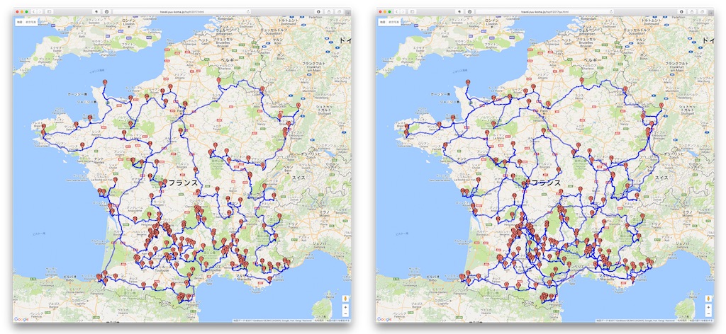
Below are the results of the conventional version vs. the quantum version. The one on the left is the program we used three years ago, and the one on the right is the one we ran using the quantum Monte Carlo method. You can see that the difference is obvious just by looking at the results. In the quantum version, the route in the southwestern part of France, where many beautiful villages are concentrated, is messed up.
I’ll publish the site which reflects the result of the optimization route of the quantum version, but it may be because json is heavy.
最適化ルート量子版:フランスの美しい村巡り 最適ルート2017年
However, you may need to understand the theory a little better to define the appropriate parameters.
The advantage of quantum annealing is that the ground state used here is relatively stable against various kinds of disturbances. For example, if the temperature is sufficiently low for the energy gap between the ground state and the first excited state, the temperature effect (thermal disturbance) can be neglected, but if the energy gap is small, the temperature effect becomes non-negligible, i.e., the transition from the ground state to the excited state becomes non-negligible. In other words, the transition from the ground state to the excited state becomes negligible.
Therefore, for a more rigorous calculation, the level of the parameters should be determined by balancing the temperature and the energy gap of the system, but this was not sufficiently taken into account in this case. There would have been room for more careful tuning in this area. Unfortunately, we did not have the time or the ability to explore this far.
However, even though it failed this time, if I were to mention the superiority of quantum Monte Carlo again, it would be that even if the number of bits increases, the number of calculations is, after all, the number of Monte Carlo simulations per simulation times the number of annealing attempts, so the time to complete a calculation does not increase exponentially. This means that the time to complete the calculation does not increase exponentially even if the number of bits increases. This is a big difference compared to conventional calculation methods, and this is also pointed out in the Google and NASA papers.
I wish there was a quantum Monte Carlo library -> there is!
On the other hand, I thought that there might be room to devise Python code. For example, I thought it would be nice to have the Tensor Flow quantum Monte Carlo library, which is a machine learning library published by Google, since Google is actively researching quantum computers. But it seems that there is none at the moment.
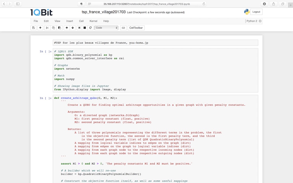
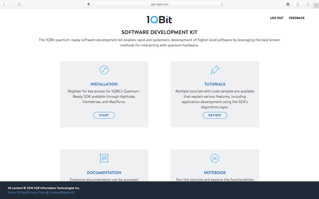
But instead, I discovered that the example company 1Qbit has secretly released this SDK.
1Qbit SOFTWARE DEVELOPMENT KIT: 1Qbit SOFTWARE DEVELOPMENT KIT
If you read the aforementioned white paper carefully, you’ll see that the research here also used this SDK.
You need to register an account to use this SDK, but it’s free.
ということでサインインして早速使ってみようとしたのですが、ローカルの端末にはインストールできませんでした。なぜインストール出来ないのかは、どうやらGithub上にはもうこのSDKのリポジトリが存在しないからみたいです。しかし、[highlight]「 1QBit’s interactive Jupyter Notebook」[/highlight]を利用すればブラウザ上でこのSDKを利用できるようなので、こちらで試してみることにしました。
Some sample code is included. The python library needed for analysis is already installed, which is convenient. And it’s much crisper and easier to use than I expected. If you try to run these sample codes, you can feel the usability immediately.
Note that once you log off, the newly created file will be lost, so you need to download it from the server before you log off. The downloaded files may have .html or .json extensions, but you can remove these extensions and change them to .py or .ipynb after downloading. When you log in again, just upload the .py or .ipynb file and you’re good to go.
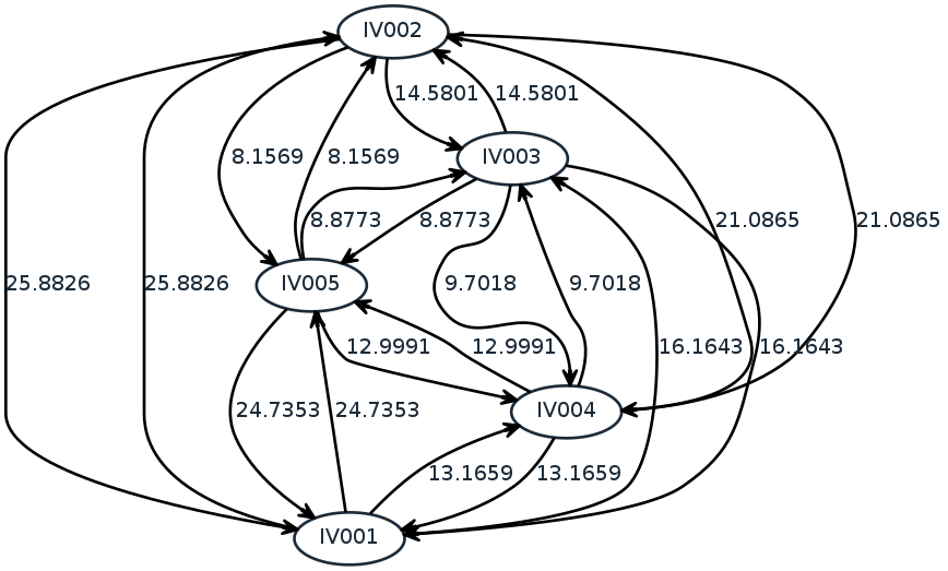
さて巡回セールスマン問題を考える上で、1Qbitがサンプルとして公開しているpythonの中で、今回最も参考になりそうだったのが、前述した[highlight]「Finding Optimal Arbitrage Opportunities Using a Quantum Annealer」[/highlight]というホワイトペーパーで実際に用いられたコード。このペーパーの対象は為替のアービトラージの最適化ですが、各為替間のレート=コンバージョンレートがちょうど村の間の地図に相当するので、入力データをコンバージョンレートから距離情報に置き換えれば、巡回セールスマン問題に適用できるかもしれないと考えました。とりあえず適当に5地点のデータ(IV001からIV005、数字は適当)を入れて、サンプルプログラムどおりにチャート図を作ったのがこちら。
ただし、このペーパーで使用している目的関数の中では、すべての村は1回のみ訪れるという制約条件=ペナルティー項は考慮されていますが、[highlight]「1つの閉じたルートにすべての村が含まれる」[/highlight]という制約部分閉回路(閉集合)を除去するためのペナルティー項が入っていません。とはいえ、この最後の条件を自作して反映するのは厳しいと思ったので、部分閉回路の解をあったとしても気にしないで、とりあえず1Qbitの為替アービトラージのコードの中で、入力データは美しい村間の移動距離、そして最適化のための目的関数およびペナルティ項は以下のように設定してプログラムを動かすことにしました。
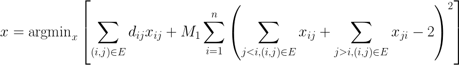
We decided to improve only the code where it corresponds to this part and use the rest as it is.
しかし、まず試しに適当なデータを利用して、5個の村バージョンで計算しようとしましたが、いろいろ試しても「もっともらしい解はない!(No feasible solutions found!)」の表示しか出ないで結局挫折。このSDKにあるminimizeという関数では、どうやら村間の移動の「向き」も区別されるようで、したがって仮に解が見つかったとしても、時計回りおよび反時計周りルートの2つ最適解が存在するため、なのでしょうか、こんな簡単が問題でも解けないみたいなのです。
Of course, it may be due to my own lack of understanding, but in any case, the SDK of this 1Qbit has just been launched. In any case, this SDK of 1Qbit has just been launched, and the sample of traveling salesman problem by quantum annealing using this SDK has not been released yet. However, we can say that traveling salesman problem is the most representative example of quantum annealing application, so let’s hope that someone will release the sample code by using this 1Qbit SDK in the near future. Of course, I also hope that more researches on other new applications will be done.
Finally, I would like to introduce the following article with such expectations. Gather round, physics graduates!
wired.jpより:人工知能がもたらす「新しいエンジニア」の時代には、物理学者がテック業界を支配する
Summary, Impressions, etc.
So I studied about “quantum computer by quantum annealing method”, which will continue to be a hot topic in 2017, and actually experienced its effect. I realized that it takes too much time to reproduce with conventional computers and with the quantum Monte Carlo method.
We were able to learn concretely that research on the application technology of quantum computers, not only in terms of hardware but also in terms of software, has progressed more than expected. As for the software side, various ideas are expected to emerge in the future, mainly from 1Qbit, the company introduced here. We hope that the 1Qbit SOFTWARE DEVELOPMENT KIT will be further expanded in the future.
And this time, in order to understand this quantum annealing, I studied statistical mechanics again after a long time, but it didn’t take me long time to remember it because I had studied it well when I was a university student. Therefore, I could understand this quantum annealing without much trouble.
統計力学は、統計学の理解だけでなく、最近流行りの機械学習の理論にも関連することが多いので、予想外に金融の仕事上でも役立っています。今更ながら、よい学問を専攻したと満足しています。